Because in probability based statistics it is always possible to make probability-statements about the same future observations (i.e. make predictions) on basis of different probabilistic theories (or methods) that cannot be true at the same time.
So as an example, we can use lots of sets of probabilistic assumptions and an infinity of estimation methods and surely claim that the probability of rain tomorrow is 0.4, 0.5 or any other probability value. At the same time it is impossible to prove one of the claims or theories definitively wrong.
So it seems to be impossible to collect empirical stochastic knowledge in a Database. In our reasoning there is no stochastic empirical knowledge and a database containing empirical results that are based on stochastic models could include an infinite number of conflicting statements.
One of the major advantages of emergent-law-based statistics therefore is the fact that emergent laws and the simple prediction rule “predict that a pattern that always was true in the past also will become true the next time” cannot result in conflicting predictions. So it becomes possible to collect consistent empirical knowledge in form of emergent laws in databases.
See the power of the resulting KnowledgeBases in the following example:
(Click on the image for fullscreen.)
KnowledgeBase Explanation
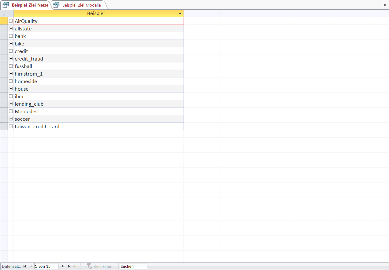
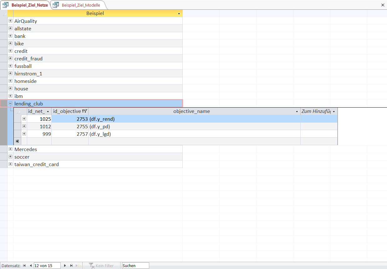
The KnowledgeWarehouse in this example gives an overview for a few databases from a wide variety of sources and topics ranging from technical and environmental datasets to economic and business data.
Examples include soccer games with betting odds ('soccer'), gas-sensor measurements ('AirQuality'), returns and customer information by the P2P-Lender (LendingClub), insurance claims from customers ('allstate'), testing times for cars ('Mercedes'), departure of employees ('ibm'), credit scoring and risk calculation ('credit') and many more.
In this explanation we will examine the datasets 'soccer', 'AirQuality' and 'lending_club' for a small glimpse into the power of a KnowledgeWarehouse.
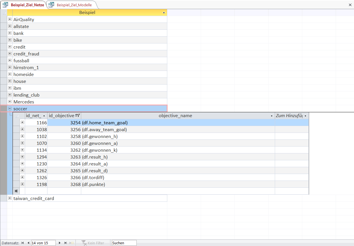
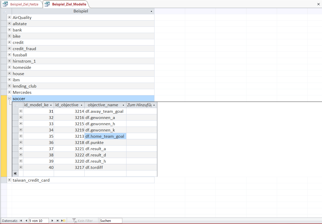
The dataset 'soccer' consists of major european soccer leagues (like Germany, Spain, UK,...) from 2008 to 2016 with match information and betting odds by up to 10 providers. (source).
The dataset has some "interesting" variables that can be predicted.
Among them are home_team_goal (number of goals by home team), gewonnen_h (1 if home team wins, 0 if not), gewonnen_k (1 if tie, 0 if not), result_h (percentage return for betting on the home team) and other variables.
In the KnowledgeWarehouse, numerous Objects, which are part of KnowledgeNets, are associated to an objective (in this case to home_team_goal).
These objects, in some way or another interesting, have been selected by our KnowledgeNet-Algorithm beforehand.
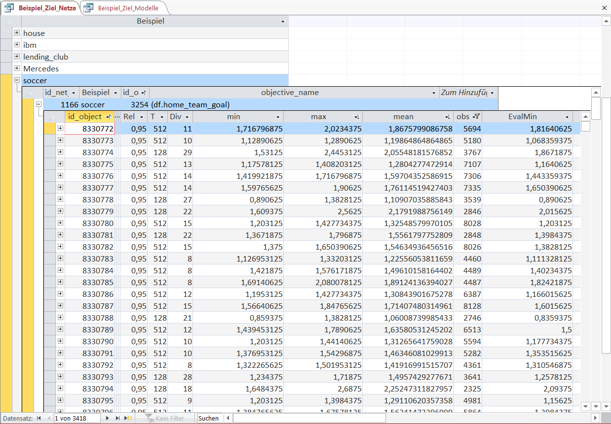
Objects have the property that they emergent-always had a different "mean" concerning one of the objectives relative to all other Objects of similar size (in their "peergroup").
As we will see later, an Object is simply a rule to select certain observations based on some properties.
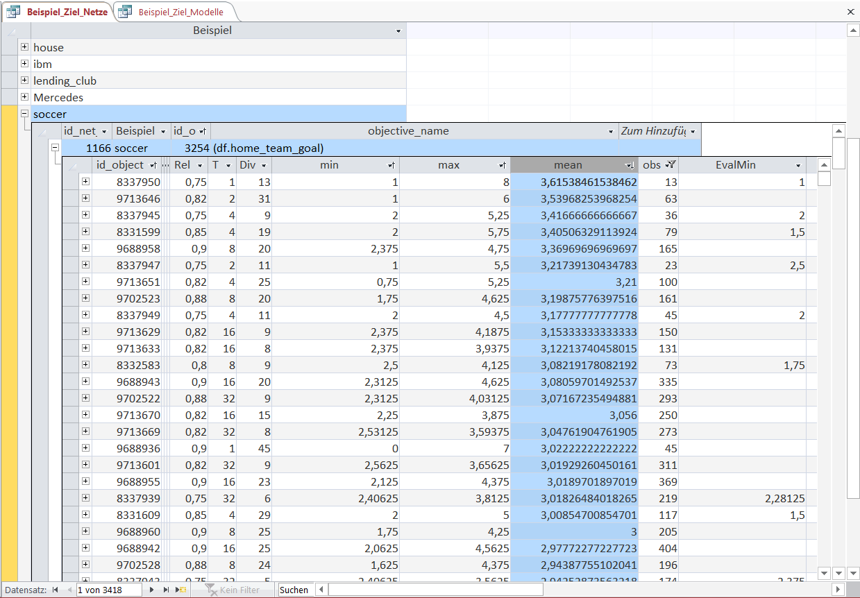
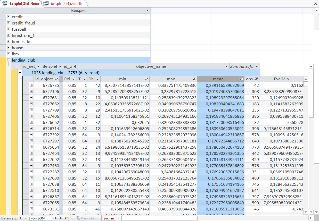
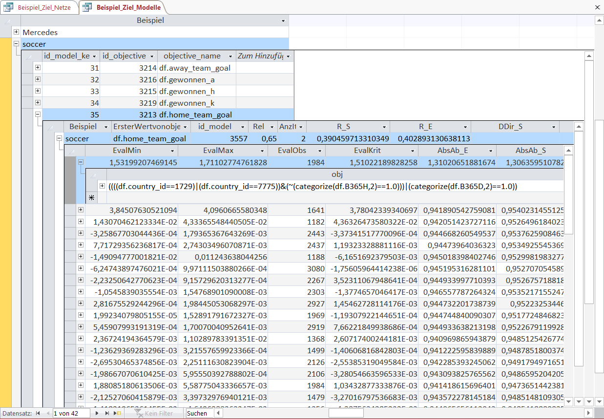
Each Object (identified by its id_object property) has certain characteristics displayed in the table:
The field 'mean' is the arithmetic mean of the variable home_team_goal for the selected observations, i.e. the value 1.867 in the first row means that the home team on average scored 1.867 goals in the selected games.
The field 'obs' indicates the number of games selected by the Object-rule: 5694 games.
'Rel' means Reliability and is the target rate for how many Emergent Laws are falsified over time, i.e. in this case how many Objects remain emergent-different from one another in the KnowledgeNet.
The Emergent Law has the properties 'T' and 'Div', which is the size of the set of emergence and the Degree of Inductive Verification, i.e. the number of confirmations in non overlapping windows of 'T'.
'min' and 'max' is the minimum and maximum arithmetic mean in a rolling window of size 'T' of the Object for the specific variable (here home_team_goal).
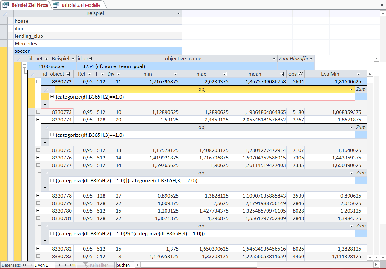
The Object-rule that selects certain observations (games) is shown in this graphic for a few selected Objects.
Of course every Object-rule only requires information for the selection that are always available at each point in time (no Look-Ahead Bias).
Note that 'categorize()' is an expanding quantile function with a certain game characteristic and the number of equally sized quantiles as the parameters. For the first Object-rule 'B365H' is the betting odd by bwin for a victory by the home team and '2' splits the betting odd into 2 quantiles (upper half and lower half).
The '==1.0' then selects the lower half ('==2.0' would be the upper half).
For a different object the betting odd is split into 3 quantiles and the lowest third ('==1.0') is selected.
Different quantile selections can be combined with logical operators like AND (&), OR (|), NOT (~).
The Objects can then be sorted or filtered in order to select interesting Objects, gain information about the dataset and what the driving factors are for certain variables of interest.
In this case the Objects are sorted in descending order of their 'mean' but for brevity other orders with different characteristics like 'min'/'max' or filters for certain keywords in the Object-rule are not shown.
The first Object has a 'mean' of 3.615 meaning that on average the home team scores 3.615 goals in each match. This Object-rule selects 13 games.
Let us look at the Object-rule and see how to identiy matches with such a high number of goals for the home team.
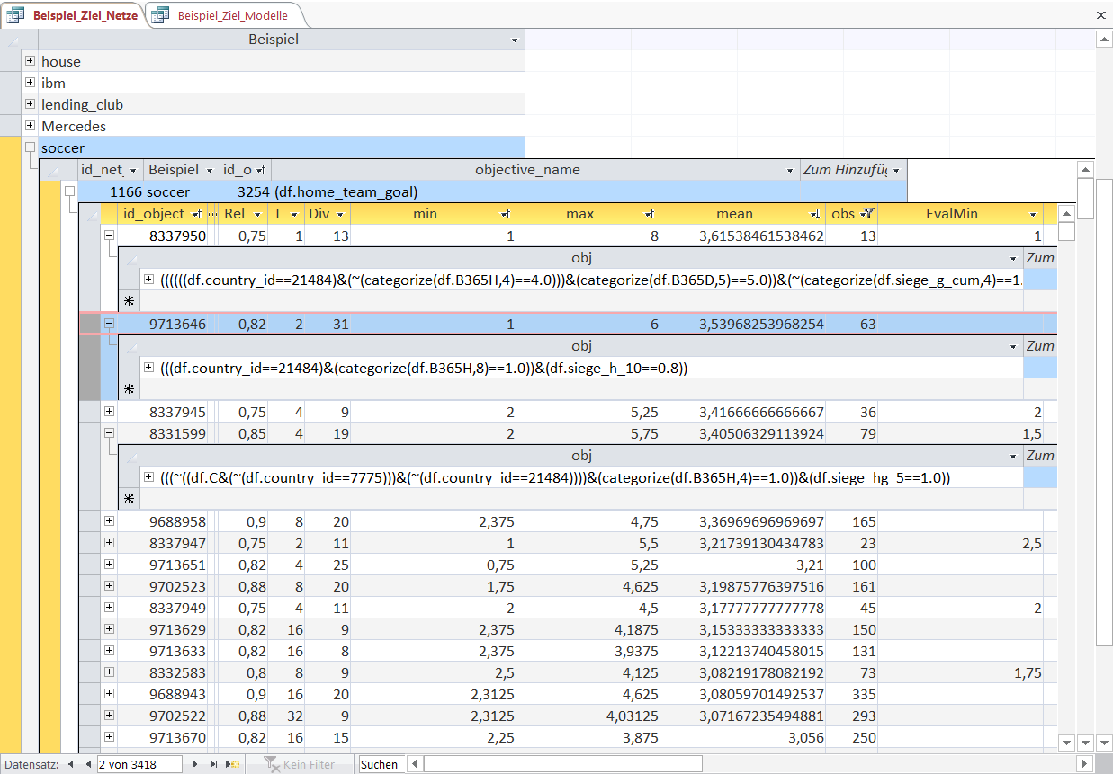
The first object is a little bit complicated to interpret at first sight.
A little part of the Object-rule is missing due to the displayed cell width but in oder to get the point the displayed part should suffice.
The country_id of 21484 refers to the German soccer league Bundesliga.
The next part selects not (~) the games with a high betting coefficient for the home team (deselects the expanding top quartile), i.e. you would not receive much payout for a victory bet on the home team (home team is favourite team).
Then the matches with the lowest expanding quartile of cumulated victorys for both teams are deselected.
The 'min' of 1 shows that in each of these 13 games a minimum of 1 goal was scored by the home team and a maximum of 8 goals.
The second Object '(((df.country_id==21484)&categorize(df.B365H,8)==1.0))&(df.siege_h_10==0.8))' with a mean of 3.53 selects the matches in Germany with the lowest expanding percentile (8 --> 12.5%) betting coefficient (low payout) and the teams with 8 victorys of the last 10 games.
Both Object-rules obviously select matches where the home team is the clear favourite and has a much higher skill level compared to the away team thus resulting in the high number of goals by the home team.
And with a KnowledgeWarehouse it is possible to discover the determining factors - as we will see for a wide variety of datasets.
(Note: a 'country_id' of 7775 refers to the Spain soccer league Primera División)
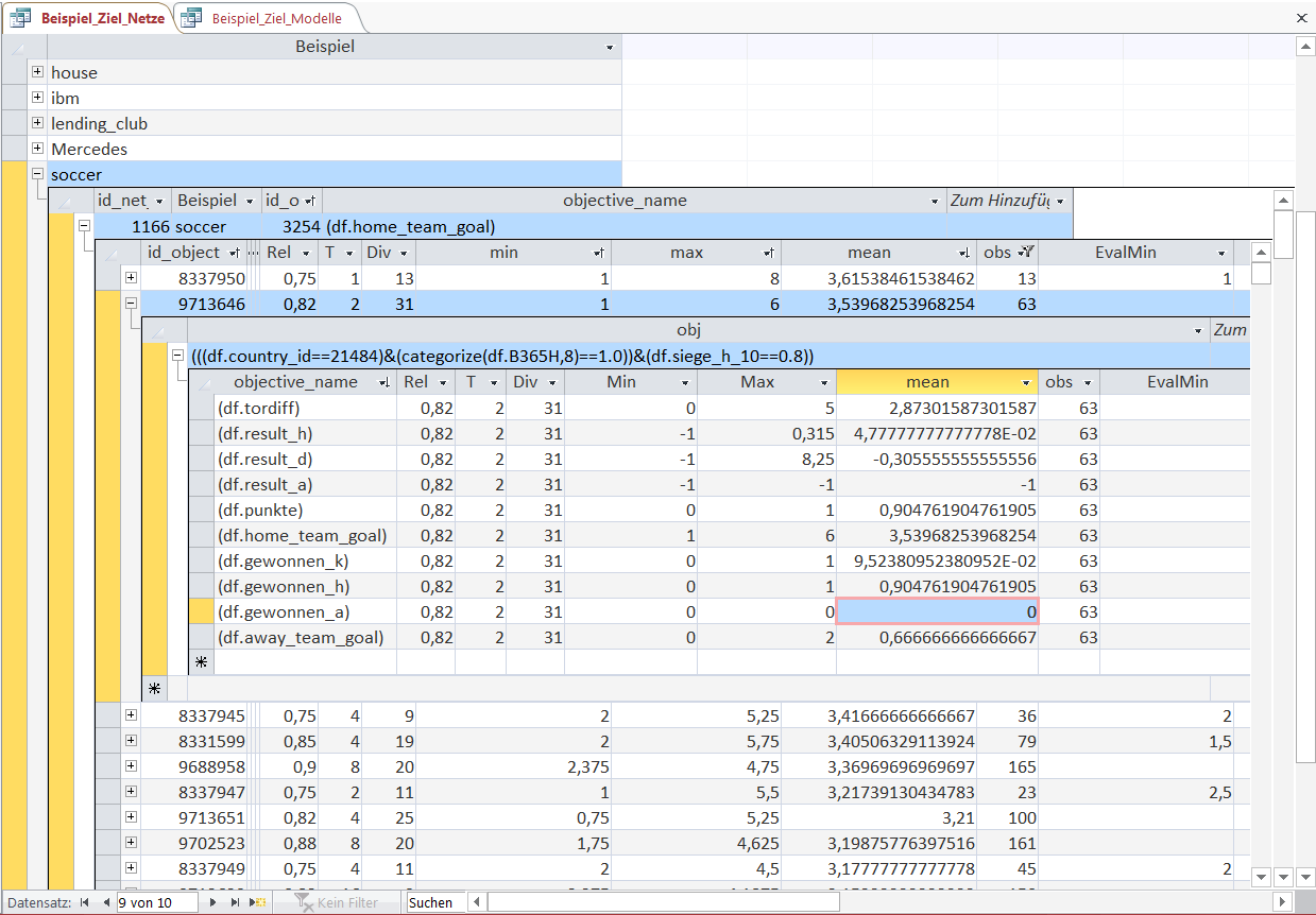
A very powerful feature of the KnowledgeWarehouse is to look at different variables (objectives) for the same Object.
In this case we examine the second object.
It is not surprising that games with such a high number of goals for the home team result in 0 won games for the away team ('gewonnen_a'). The home team wins 90.47% of these games ('gewonnen_h') and the remaining 9.52% end in tie ('gewonnen_k').
On average home team wins by a margin of 2.87 goals ('tordiff'). The minimum margin was 0 (the tie games) and the maximum margin was 5 games ('min' and 'max').
But nevertheless very interesting is that if you use this Object-rule to bet on the home team you would make 4.7% with these bets on average.
Unfortunately a return of 4.7% is below the transaction costs for placing soccer bets but with the KnowledgeWarehouse it is easily possible to identify betting strategys with a positive return after transaction costs.
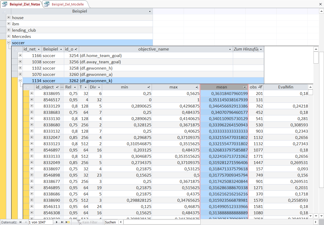
Now let us look at a different objective - in this case 'gewonnen_k', i.e. a binary variable (1 if a tie, 0 for the rest).
This time the Objects are again sorted in descending order of their mean. A mean of 0.36 in the first cell simply means that 36% of the games selected by this Object-rule end in a tie.
As usual in Machine Learning, the dataset is split into two parts (in-sample and out-of-sample data). The fields 'min','max','mean' are all calculated with in-sample data.
Now let us look at the out-of-sample equivalents 'EvalMin', 'EvalMax' and 'EvalMean'.
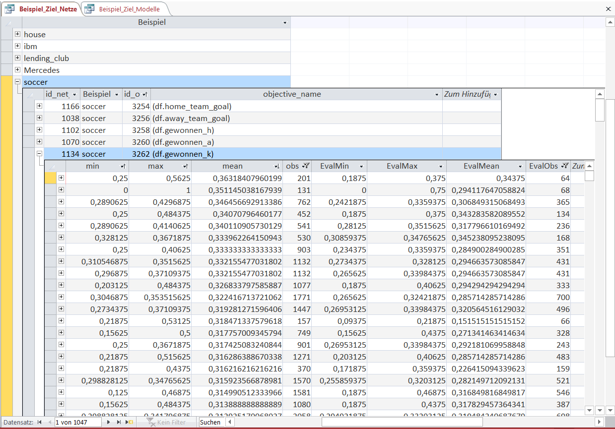
If you look at the order created by 'mean' and the order of 'EvalMean' it is not always correct, in a sense that 'EvalMean' is constantly decreasing.
This corresponds to the intially explained Reliability. Some of the Emergent Laws are falsified over time, i.e. the Objects do not remain emergent-different from one another in the KnowledgeNet, thus resulting in a "wrong" order of 'EvalMean'.
Nonetheless the value 'EvalMean' and the approximate range given by 'EvalMin' and 'EvalMax' transfers reliably and accurately between in-sample and out-of-sample data.
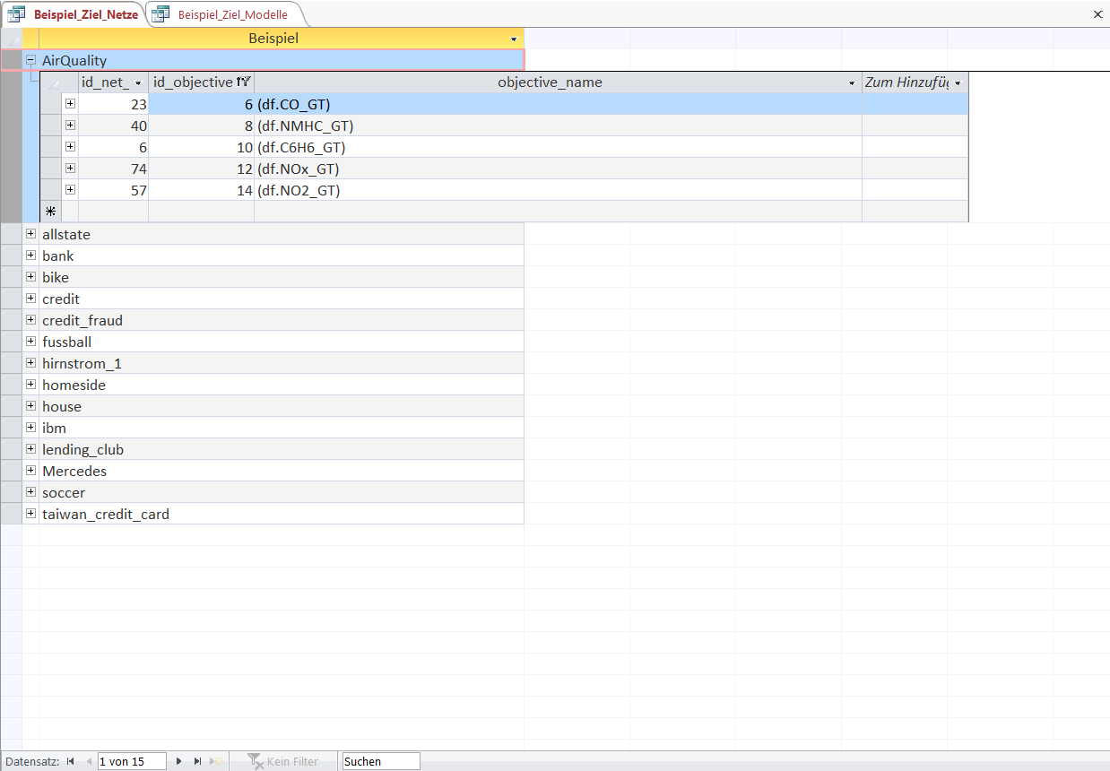
The next example that we will explore is the technical dataset 'AirQuality'.
It contains hourly measurements of a gas multisensor device and a certified analyzer in an Italian city (source).
One common target is to predict the very precise concentration measurements of 'CO_GT' (Carbon Monoxide in mg/m^3), 'NMHC_GT' (Non-Metanic Hydrocarbons in microg/m^3), 'C6H6_GT' (Benzene in microg/m^3), 'NOx_GT' (Nitrogen Oxides in ppb) and 'NO2_GT' (Nitrogen Dioxide in microg/m^3) recorded by the expensive certified analyzer only with the recordings of the cheap multisensor device.
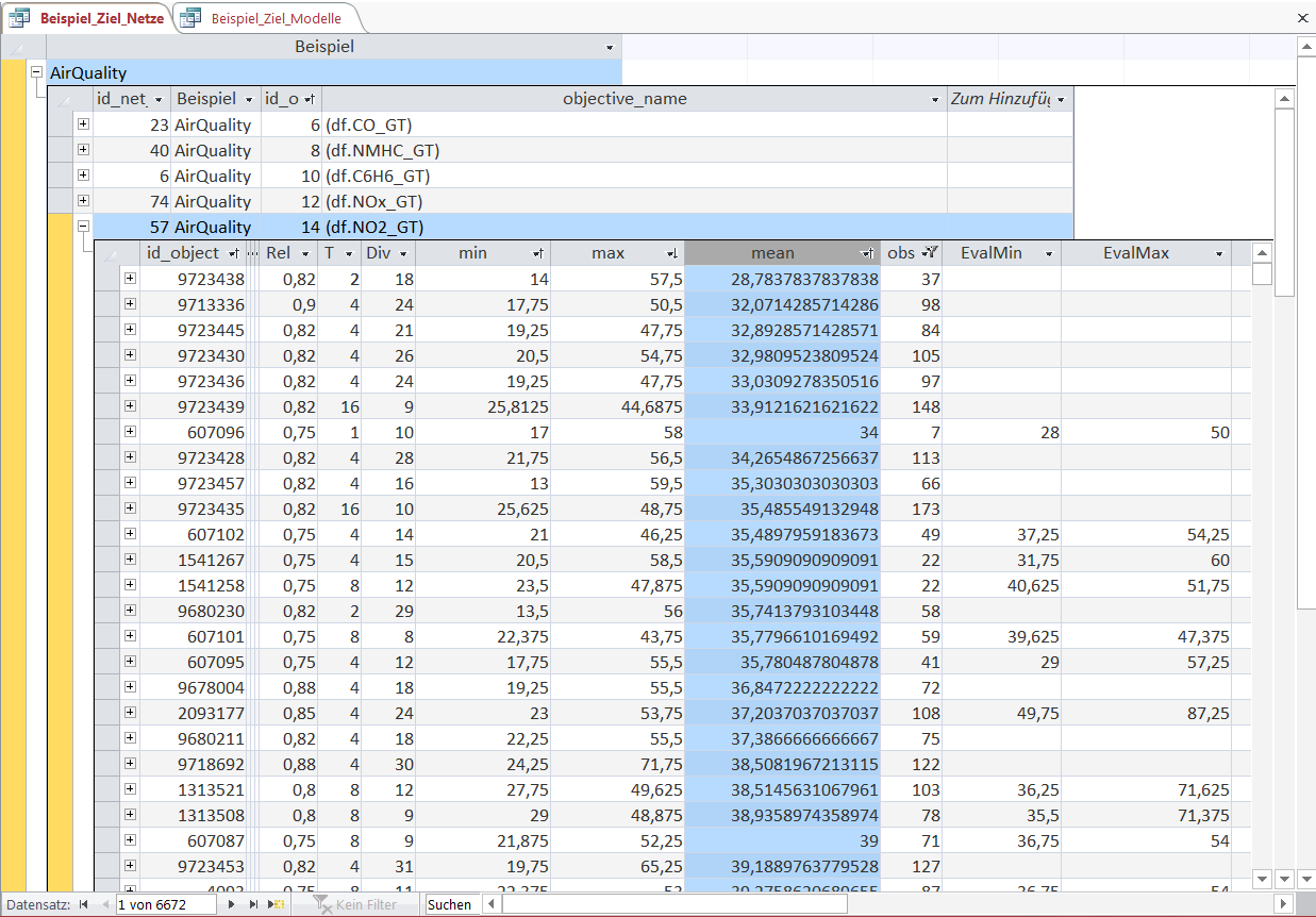
In this overview we see the Objects for the Nitrogen Dioxide concentration ('NO2_GT' measured in microg/m^3 by the expensive certified analyzer) sorted in ascending order of their mean.
The meaning of the fields is the same as that previously explained in the 'soccer' example - except that the variable of interest is not soccer goals, betting odds or match results but gas concentrations.
And an Object-rule selects points in time instead of soccer matches.
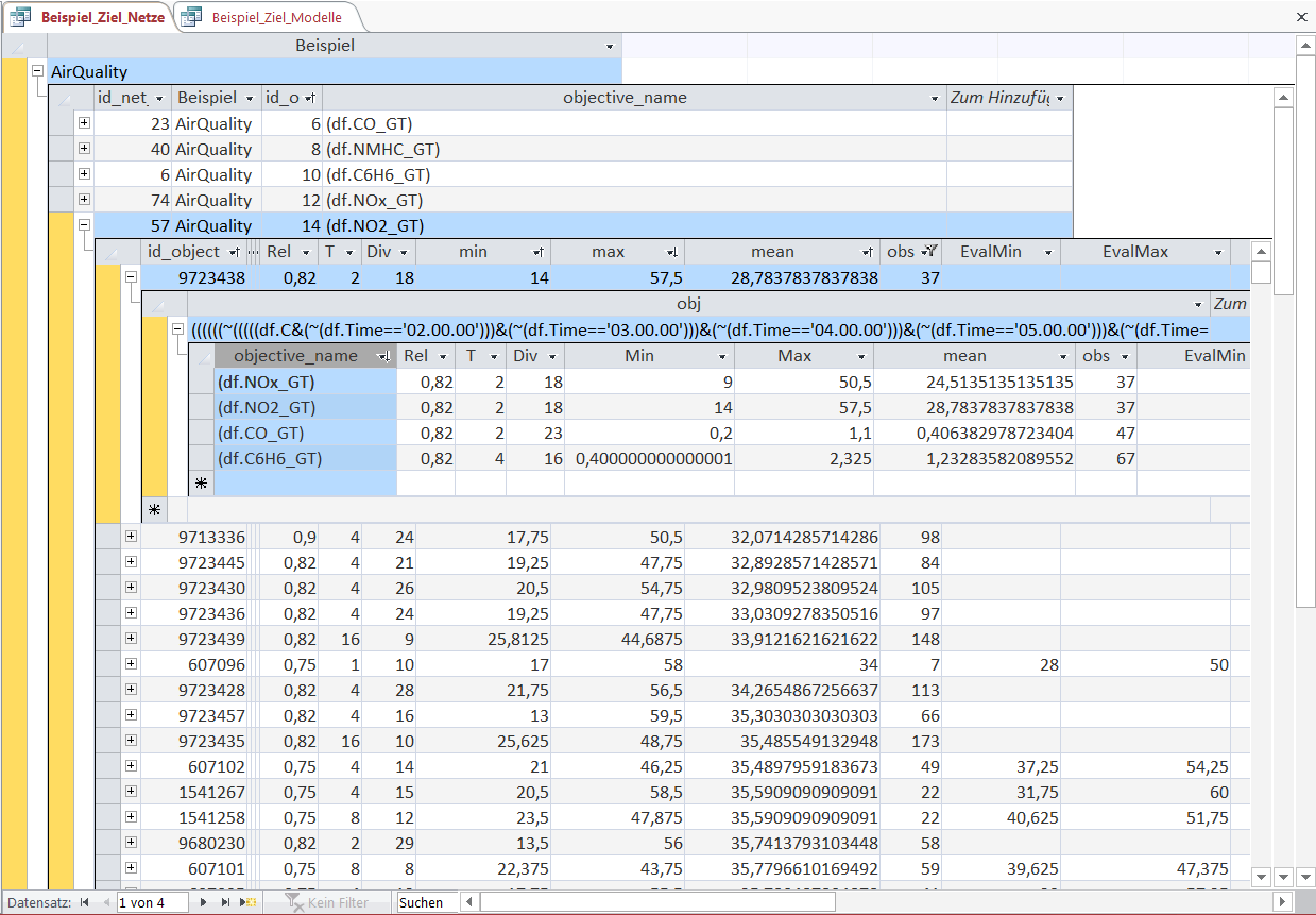
For the sake of brevity we only examine the Object with the lowest average 'NO2'-concentration, its defining Object-rule and its values for different variables (i.e. gas concentrations).
The selected Object-rule is in full length:
((((((~(((((df.C&(~(df.Time=='02.00.00')))&(~(df.Time=='03.00.00')))&(~(df.Time=='04.00.00')))&(~(df.Time=='05.00.00')))&(~(df.Time=='06.00.00'))))&(categorize(df.PT08_S1_CO,8)==1.0))&(categorize(df.PT08_S2_NMHC,7)==1.0))&(~(categorize(df.PT08_S2_NMHC.diff(),4)==3.0)))&(categorize(df.PT08_S5_O3,10)==1.0))&(categorize(df.PT08_S5_O3.diff(),8)==4.0))
From the Object-rule it is directly evident that the 'Time' of the measurement is a very essential factor for the 'NO2'-concentration. This is linked to the changing traffic volume over the course of a day.
The Objet-rule selects the time between 2:00 a.m. and 6:00 p.m. (the double negation with ~ and the multiple braces) due to the very low traffic volume.
The next parts of the rule select the observations based on the sensor measurements:
lowest expanding 12.5%-quantile of the PT08_S1 sensor (tin oxide sensor); lowest expanding 14.29%-quantile of the PT08_S2 sensor (titania sensor); not the expanding 50%-75%-quantile of the PT08_S2 sensor as the difference to the preceeding hour; lowest expanding 10%-quantile of the PT08_S5 sensor (indium oxide sensor); lowest expanding 12.5%-quantile of the PT08_S1 sensor (tin oxide sensor); expanding 37.5%-50%-quantile of the PT08_S1 sensor as the difference to the preceeding hour

Now we can analyse the results for the other variables in the dataset with the same Object-rule applied.
This immediately gives you an idea how the lowest 'NO2'-concentration is connected to the other gas concentrations.
(In order to compare the values it would be necessary to know the levels of the different gas concentrations but in this small example the levels are only presented and not shown in the KnowledgeWarehouse).
It is not surprising that the 'NOx'-concentration on average is very low when the 'NO2'-concentration is also low (overall mean of 'NOx'-concentration is 214.37 ppb).
The average 'CO'- as well as the 'C6H6'-concentration are also at a relatively low level (overall average 'CO'-concentration is 2.18 and 'C6H6'-concentration is 1.73).
So it seems to be that the air pollution for this Object-rule is very low for all analysed pollutants.
As the last example for a KnowledgeNet in the KnowledgeWarehouse we will examine the loan dataset of the P2P-lending platform LendingClub (source).
LendingClub is an online marketplace where people can borrow money from other individuals that are willing to invest. The complete loan agreement (pricing/legal structure etc...) is handled by LendingClub.
The dataset contains complete loan data from 2007 to 2015 with information like (requested amount, interest rate, purpose, term, personal information of the borrower etc). For our purposes we only analyse the loans with a term of 3 years.
The target variables that are very useful for investing and knowledge are the return ('y_rend'), the empirical rate of default ('y_pd') and the loss given default ('y_lgd').
In this case 'y_rend' is the total return for a 3-year loan (i.e. money received over time/money given at the beginning of loan).
The empirical rate of default 'y_pd' is a simple binary field indicating whether the borrower missed payments and defaulted (then 1) or repaid the credit accordingly (then 0).
If a borrower defaults, LendingClub liquidates the provided collaterals. The variable 'y_lgd' is the percentage of how much an investor looses based on his invested amount after considering the borrower's securities ([money received over time - loan amount]/loan amount).
We can now go into more detail for the variable 'y_rend' - the total return of a loan.
The Objects are sorted in descending order of their mean, i.e. a 'mean' of 23.9% is the Object with the highest average return (please remember, this is the total return over 3 years not the 1-year return).
But nevertheless, the displayed returns are still sizeable returns. As a side note: the highest return of 23.9% holds perfectly true for the out-of-sample data with a return of 22.1%.
Please also note that the minimum return ('min' and 'EvalMin') for the highest performing Object never dropped below 8.7% within-sample and 11.6% out-of-sample. This also holds true for almost all displayed Objects.
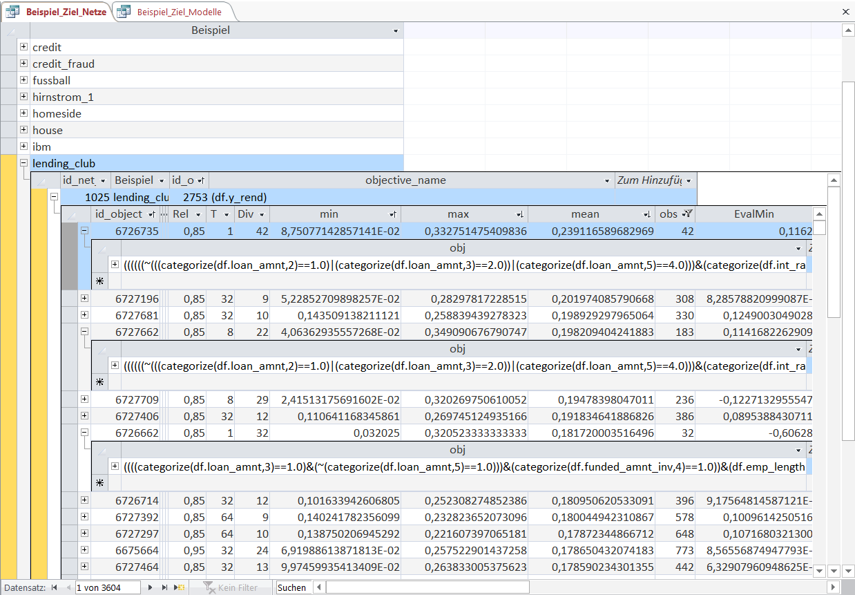
The first Object-rule selects the loans based on the requested loan amount, the interest rate and the employment length:
the highest expanding 20%-quantile of requested loan amount 'loan_amnt' (negation at the beginning); the highest expanding 20%-quantile of interest rate 'int_rate' and an employment length of 10 years or more.
In general, Object-rules always select points in time. However the concrete data entry obviously varies for the different datasets.
For example in the previous datasets, the Object-rules selected soccer machtes or points in time for sensor measurements. In this case the Object-rule selects individual loans.
This has significant consequences as every Object-rule can be directly used as a decision rule to construct a loan portfolio for investors.
The decisions made by the Objects can be used to follow the principle of T-Dominance:
If you have the choice between two decision rules choose the rule that always led to a better result after T decisions. (a longer explanation of T-Dominance).
After a quite thorough look on various KnowledgeNets we focus our attention on Models in the KnowledgeWarehouse.
Models are built on top of KnowledgeNets in order to make "classical" point estimates of a certain variable. In this sense KnowledgeNets provide a solid foundation for a multitude of different possibilities with Models just being one of the straight-forward applications.
Models use the Objects in the KnowledgeNet to find estimation heuristics to make point estimates that emergent-always led to a better prediction performance (in terms of a certain criteria like mean absolute prediction error, logarithmic prediction error, mean squared prediction error,...).
To better understand the process of Model-building we will look at a model for the number of scored goals by the home team in the soccer dataset.
A deeper explanation of the Model-building-process can be found in the Notebook: The process of emergent law based model building.
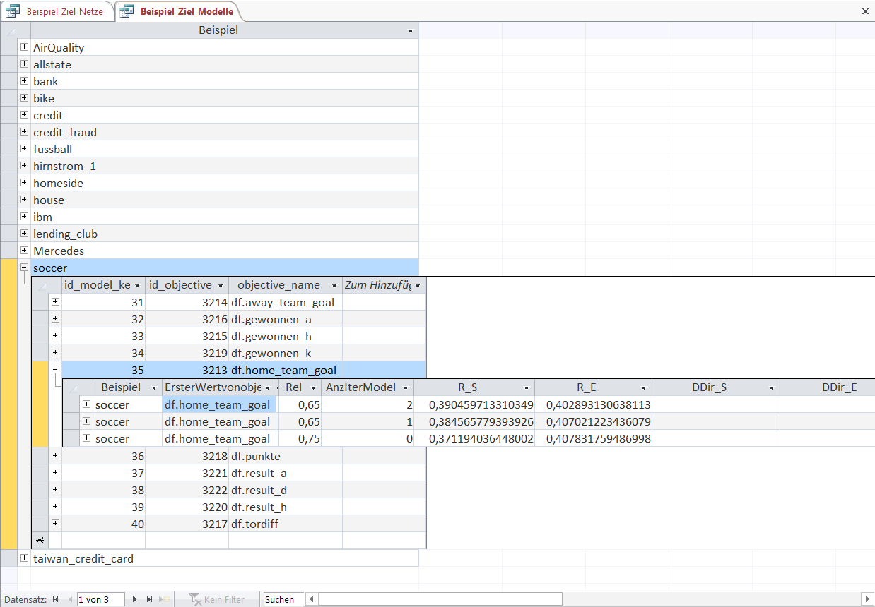
Since there are multiple Models in the KnowledgeWarehouse, this overview shows the best found models for predicting the number of goals by the home team ('home_team_goal').
In this overview the best models are selected due to their within-sample correlation coefficient ('R_S'). As you can see from the out-of-sample correlation (shown in column 'R_E') the models performed as expected.
The overview shows models of 3 different model-types denoted by the value in the 'AnzIterModel' column.
A value of '0' is a very simple and fast benchmark model that works with a list of heuristics (expanding-T-means, expanding-Least-Square-Estimators etc.) to find a model that always improved a prediction error metric.
The values '1' and '2' show model iterations that use the Objects of the KnowledgeNets together with a list of heuristics (more about it later).
The meaning of 'Rel' (Reliability) for Models is similar to its meaning for KnowledgeNets.
For Models it is the target rate for how many Emergent Laws in the Model are falsified over time, i.e. in this case how many Emergent Laws improve the prediction out-of-sample according to some metric.
We will have a look at the first displayed model.
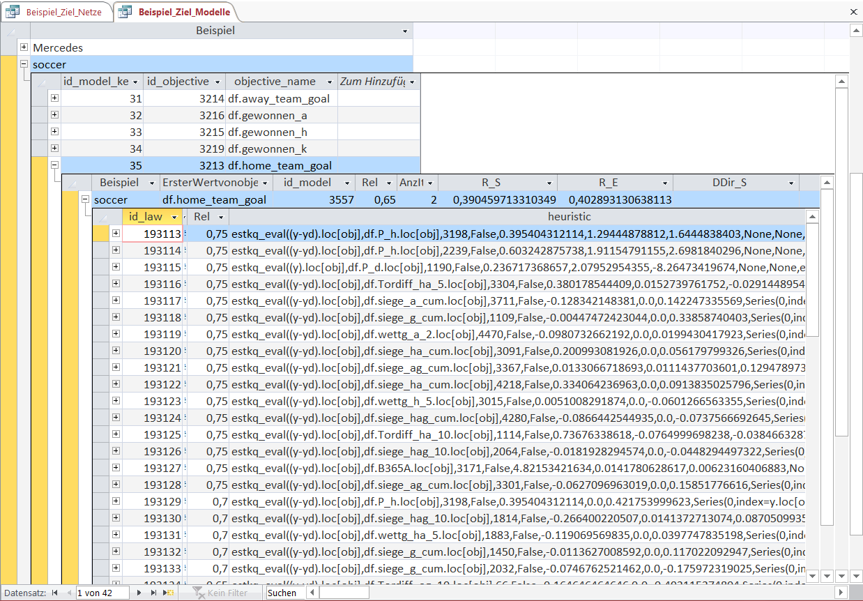
Each Model consists of a sequence of estimation heuristics that are applied to Objects of a KnowledgeNet.
It is an Emergent Law that every Object-heuristic combination improves the prediction accuracy according to some specified metric.
The dropping Reliability shows that the aforementioned model iterations '1' and '2' reduce the necessary Reliabilty for the Emergent Laws.
We can now examine the Object-heuristic combinations for a few selected entries in the Model to explain the purpose and functionality of an Object-heuristic combination.
In the first step an Object-rule is used to select certain entries in the dataset (here soccer matches). Then the heuristic function (here beginning with 'estkq_eval') is used to make a point estimate for the selected observations.
A model is simply a sequence of these Object-heuristic combinations.
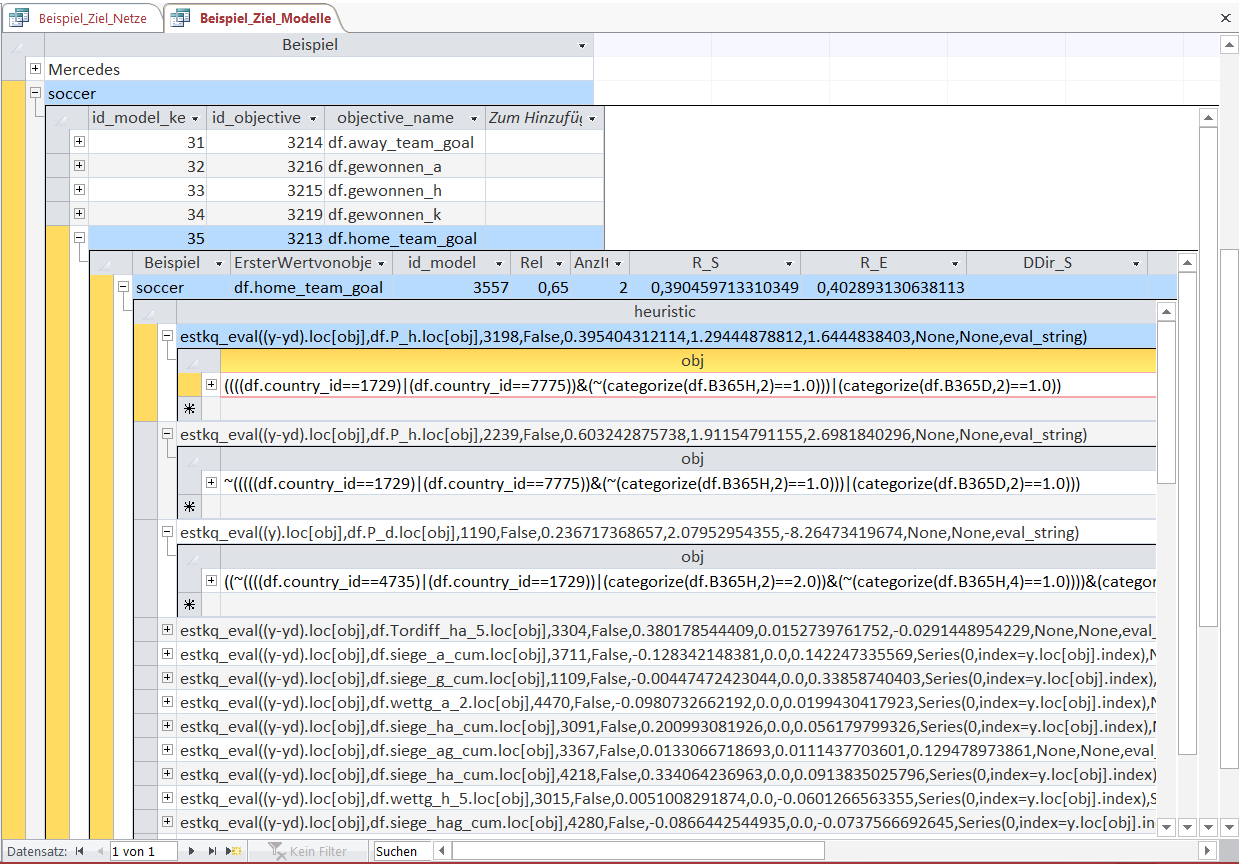
In the displayed table you can see 3 Object-heuristic combinations in detail. The meaning of Object-rules is the same as in the KnowledgeNets.
The first heuristic function beginning with 'estkq_eval' is a simple expanding-least-square-estimator.
In this case the variable 'P_h' (the implicit winning probability of the home team calculated with the betting odds) is used as the regressor to predict the number of home team goals ('y').
The values 0.39 and 1.29 show the mean of home team goals and the mean of the winning probability for the observations selected by this Object-rule.
The value 1.64 is the regression coefficient, i.e. the number of goals scored by the home team rises by 1.64 for every unit of winning probability (and vice versa).
In this overview there are only expanding-least-square-estimators used but other heuristics like simple expanding mean estimators or rolling mean estimators can also be chosen by the program.
The decision which heuristic to apply for each Object-rule is taken based on the improvement of the specified error metric.
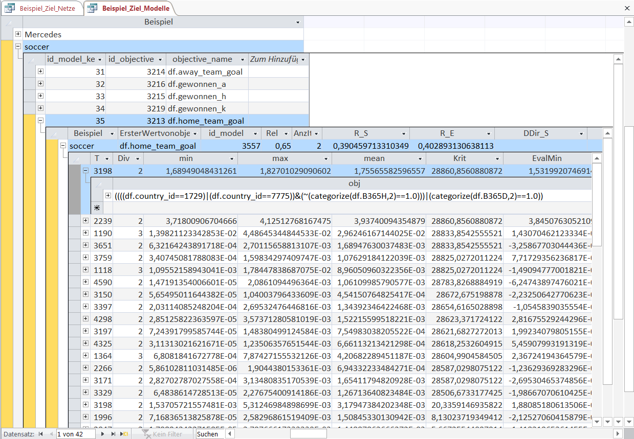
Since all Object-heuristic combinations are Emergent Laws, they share the same properties like the Objects in the KnowledgeNet.
But this time the values of 'min', 'max', 'mean' and the like are the improvement of the prediction calculated using an error metric.
Of course the Emergent Laws are also evaluated with the out-of-sample data.
A negative value in the column 'EvalKrit' shows that the Object-heuristic combination worsens the prediction performance out-of-sample.
At each step in the sequence of a model it is possible to calculate the overall error for a range of different error metrics.
'AbsAb_S' is the mean absolute prediction error within-sample ('AbsAb_E' out-of-sample). The error within sample is not monotonous decreasing because for this model the used error metric was the mean squared prediction error.
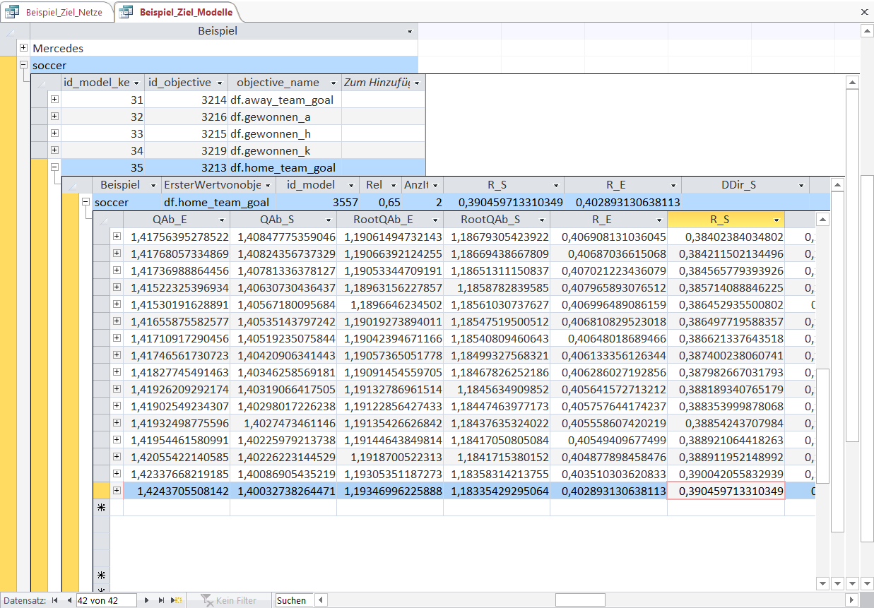
Other error metrics are the already mentioned mean squared prediction error ('QAb'), the root mean squared prediction error ('RootQAb') or the correlation coefficient ('R').
The '_S' part in the column description denotes that the criteria is calculated with within-sample data whereas the '_E' shows the out-of-sample equivalents.
The within-sample correlation of 0.39 in the top overview row corresponds to the 'R_S' value in the last row of the model (logically, the model ends after the last Object-heuristic combination).